Home >> Blog >> 什麼是 quicksort 快速排序
什麼是 quicksort 快速排序
與合併排序一樣,快速排序是一種分治算法。它選擇一個元素作為樞軸,並圍繞選擇的樞軸對給定數組進行分區。有許多不同版本的 quickSort 以不同的方式選擇樞軸。
- 始終選擇第一個元素作為樞軸。
- 始終選擇最後一個元素作為樞軸(在下面實現)
- 選擇一個隨機元素作為樞軸。
- 選擇中位數作為支點。
quickSort中的關鍵過程是 partition()。分區的目標是,給定一個數組和一個數組的元素 x 作為樞軸,將 x 放在已排序數組中的正確位置,並將所有較小的元素(小於 x)放在 x 之前,並將所有較大的元素(大於比 x) 在 x 之後。所有這些都應該在線性時間內完成。
分區算法:
分區的方法有很多種,下面的偽代碼採用了 CLRS 書中給出的方法。邏輯很簡單,我們從最左邊的元素開始,跟踪更小(或等於)元素的索引為 i。在遍歷時,如果我們找到一個較小的元素,我們將當前元素與 arr[i] 交換。否則,我們忽略當前元素。
遞歸快速排序函數的偽代碼:
/* low –> Starting index, high –> Ending index */
quickSort(arr[], low, high) {
if (low < high) {
/* pi is partitioning index, arr[pi] is now at right place */
pi = partition(arr, low, high);
quickSort(arr, low, pi – 1); // Before pi
quickSort(arr, pi + 1, high); // After pi
}
}
partition() 的偽代碼
/* This function takes last element as pivot, places the pivot element at its correct position in sorted array, and places all smaller (smaller than pivot) to left of pivot and all greater elements to right of pivot */
partition (arr[], low, high)
{
// pivot (Element to be placed at right position)
pivot = arr[high];
i = (low – 1) // Index of smaller element and indicates the
// right position of pivot found so far
for (j = low; j <= high- 1; j++){
// If current element is smaller than the pivot
if (arr[j] < pivot){
i++; // increment index of smaller element
swap arr[i] and arr[j]
}
}
swap arr[i + 1] and arr[high])
return (i + 1)
}
partition() 的說明:
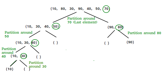
Consider: arr[] = {10, 80, 30, 90, 40, 50, 70}
Indexes: 0 1 2 3 4 5 6
low = 0, high = 6, pivot = arr[h] = 70
Initialize index of smaller element, i = -1
Traverse elements from j = low to high-1
j = 0: Since arr[j] <= pivot, do i++ and swap(arr[i], arr[j])
i = 0
arr[] = {10, 80, 30, 90, 40, 50, 70} // No change as i and j are same
j = 1: Since arr[j] > pivot, do nothing
j = 2 : Since arr[j] <= pivot, do i++ and swap(arr[i], arr[j])
i = 1
arr[] = {10, 30, 80, 90, 40, 50, 70} // We swap 80 and 30
j = 3 : Since arr[j] > pivot, do nothing // No change in i and arr[]
j = 4 : Since arr[j] <= pivot, do i++ and swap(arr[i], arr[j])
i = 2
arr[] = {10, 30, 40, 90, 80, 50, 70} // 80 and 40 Swapped
j = 5 : Since arr[j] <= pivot, do i++ and swap arr[i] with arr[j]
i = 3
arr[] = {10, 30, 40, 50, 80, 90, 70} // 90 and 50 Swapped
We come out of loop because j is now equal to high-1.
Finally we place pivot at correct position by swapping arr[ i+1] and arr[high] (or pivot)
arr[] = {10, 30, 40, 50, 70, 90, 80} // 80 and 70 Swapped
Now 70 is at its correct place. All elements smaller than 70 are before it and all elements greater than 70 are after it.
Since quick sort is a recursive function, we call the partition function again at left and right partitions
Again call function at right part and swap 80 and 90
實現:
以下是快速排序的實現:
/* C++ implementation of QuickSort */
#include <
bits/stdc++.h>
using namespace std;
// A utility function to swap two elements
void swap(int* a, int* b)
{
int t = *a;
*a = *b;
*b = t;
}
/* This function takes last element as pivot, places
the pivot element at its correct position in sorted
array, and places all smaller (smaller than pivot)
to left of pivot and all greater elements to right
of pivot */
int partition (int arr[], int low, int high)
{
int pivot = arr[high]; // pivot
int i = (low - 1); // Index of smaller element and indicates the right position of pivot found so far
for (int j = low; j <= high - 1; j++)
{
// If current element is smaller than the pivot
if (arr[j] < pivot)
{
i++; // increment index of smaller element
swap(&arr[i], &arr[j]);
}
}
swap(&arr[i + 1], &arr[high]);
return (i + 1);
}
/* The main function that implements QuickSort
arr[] --> Array to be sorted,
low --> Starting index,
high --> Ending index */
void quickSort(int arr[], int low, int high)
{
if (low < high)
{
/* pi is partitioning index, arr[p] is now
at right place */
int pi = partition(arr, low, high);
// Separately sort elements before
// partition and after partition
quickSort(arr, low, pi - 1);
quickSort(arr, pi + 1, high);
}
}
/* Function to print an array */
void printArray(int arr[], int size)
{
int i;
for (i = 0; i < size; i++)
cout << arr[i] << " ";
cout << endl;
}
// Driver Code
int main()
{
int arr[] = {10, 7, 8, 9, 1, 5};
int n = sizeof(arr) / sizeof(arr[0]);
quickSort(arr, 0, n - 1);
cout << "Sorted array: \n";
printArray(arr, n);
return 0;
}
// This code is contributed by rathbhupendra
輸出
排序數組:
1 5 7 8 9 10
使用第一個元素作為樞軸的快速排序的實現:
# include < iostream>
# include < algorithm>
using namespace std;
int partition(int arr[], int low, int high)
{
int i = low;
int j = high;
int pivot = arr[low];
while (i < j)
{
while (pivot >= arr[i])
i++;
while (pivot < arr[j])
j--;
if (i < j)
swap(arr[i], arr[j]);
}
swap(arr[low], arr[j]);
return j;
}
void quickSort ( int arr[], int low, int high )
{
if (low < high)
{
int pivot = partition (arr, low, high);
quickSort(arr, low, pivot - 1);
quickSort(arr, pivot + 1, high);
}
}
void printArray( int arr[], int size)
{
for (int i = 0; i < size; i+ +)
{
cout << arr[i] << " ";
}
cout << endl;
}
int main()
{
int arr[] = {4, 2, 8, 3, 1, 5, 7,11,6};
int size = sizeof(arr) / sizeof(int);
cout <<"Before Sorting"<< endl;
printArray(arr, size);
quickSort(arr, 0, size - 1);
cout<<" After Sorting"<
return 0;
}
輸出
排序前
4 2 8 3 1 5 7 11 6
排序後
1 2 3 4 5 6 7 8 11
快速排序分析
快速排序所花費的時間通常可以寫成如下。
T(n) = T(k) + T(nk-1) + \θ (n)
前兩項用於兩次遞歸調用,最後一項用於分區過程。k 是小於樞軸的元素的數量。 QuickSort 花費的時間取決於輸入數組和分區策略。以下是三種情況。
最壞情況:
最壞情況發生在分區過程總是選擇最大或最小元素作為樞軸時。如果我們考慮上面的分區策略,其中最後一個元素總是被選為樞軸,最壞的情況會發生在數組已經按升序或降序排序的情況下。以下是最壞情況的重現。
T(n) = T(0) + T(n-1) + \θ (n) 等價於 T(n) = T(n-1) + \θ (n)
上述遞歸的解是 (n 2 )。
最佳情況:
最佳情況發生在分區過程始終選擇中間元素作為樞軸時。以下是最佳情況的重現。
T(n) = 2T(n/2) + \θ (n)
上述遞歸的解決方案是 (nLogn)。可以使用Master Theorem的案例 2 來解決。
平均情況:
要進行平均情況分析,我們需要考慮數組的所有可能排列,併計算每個排列所花費的時間,這看起來並不容易。
我們可以通過考慮分區將 O(n/9) 個元素放在一個集合中並將 O(9n/10) 個元素放在另一個集合中的情況來了解平均情況。以下是此案例的重現。
T(n) = T(n/9) + T(9n/10) + \θ (n)
上述遞歸的解也是 O(nLogn):
儘管 QuickSort 的最壞情況時間複雜度是 O(n 2 ),比許多其他排序算法(如Merge Sort和Heap Sort )要多,但 QuickSort 在實踐中更快,因為它的內部循環可以在大多數架構上有效地實現,並且在大多數情況下真實世界的數據。QuickSort 可以通過改變主元的選擇以不同的方式實現,因此對於給定類型的數據,最壞的情況很少發生。但是,當數據很大並且存儲在外部存儲中時,通常認為合併排序更好。
快速排序穩定嗎?
默認實現不穩定。然而,任何排序算法都可以通過將索引作為比較參數來穩定。
快速排序是否就地?
根據就地算法的廣泛定義,它有資格作為就地排序算法,因為它僅使用額外空間來存儲遞歸函數調用,但不用於操作輸入。
什麼是三向快速排序?
在簡單的快速排序算法中,我們選擇一個元素作為樞軸,圍繞樞軸對數組進行分區,並在樞軸的左側和右側遞歸子數組。
考慮一個具有許多冗餘元素的數組。例如,{1, 4, 2, 4, 2, 4, 1, 2, 4, 1, 2, 2, 2, 2, 4, 1, 4, 4, 4}。如果在 Simple QuickSort 中選擇 4 作為主元,我們只修復一個 4 並遞歸處理剩餘的事件。在 3 Way QuickSort 中,數組 arr[l..r] 分為 3 個部分:
arr[l..i] 元素小於樞軸。
arr[i+1..j-1] 個元素等於樞軸。
arr[j..r] 元素大於樞軸。
我們可以迭代地實現快速排序嗎?
是的,請參考迭代快速排序。
為什麼快速排序優於 MergeSort 對數組進行排序 ?
其一般形式的快速排序是就地排序(即它不需要任何額外的存儲空間),而合併排序需要 O(N) 額外的存儲空間,N 表示可能非常昂貴的數組大小。分配和取消分配用於歸併排序的額外空間會增加算法的運行時間。比較平均複雜度,我們發現這兩種類型的平均複雜度為 O(NlogN),但常數不同。對於數組,由於使用了額外的 O(N) 存儲空間,歸併排序會失敗。
快速排序的大多數實際實現都使用隨機版本。隨機版本的預期時間複雜度為 O(nLogn)。最壞的情況也可能出現在隨機版本中,但最壞的情況不會發生在特定模式(如排序數組)中,並且隨機快速排序在實踐中效果很好。 快速排序也是一種緩存友好的排序算法,因為它在用於數組時具有良好的引用局部性。 快速排序也是尾遞歸的,因此完成了尾調用優化。
為什麼 MergeSort 比 QuickSort 更適合鏈接列表?
在鍊錶的情況下,情況不同主要是由於數組和鍊錶的內存分配不同。與數組不同,鍊錶節點在內存中可能不相鄰。與數組不同,在鍊錶中,我們可以在 O(1) 額外空間和 O(1) 時間的中間插入項目。因此可以實現歸併排序的歸併操作,而不需要額外的鍊錶空間。 在數組中,我們可以進行隨機訪問,因為元素在內存中是連續的。假設我們有一個整數(4 字節)數組 A,讓 A[0] 的地址為 x,那麼要訪問 A[i],我們可以直接訪問 (x + i*4) 處的內存。與數組不同,我們不能在鍊錶中進行隨機訪問。快速排序需要大量此類訪問。在鍊錶中訪問第 i 個索引,我們必須將每個節點從頭到第 i 個節點,因為我們沒有連續的內存塊。因此,快速排序的開銷會增加。歸併排序按順序訪問數據,對隨機訪問的需求較低。